Expectation Maximization
Last updated on 02-15-2018.
Table of Contents
- Introduction: Density estimation
- Jensen Inequality
- EM Algorithm Formalization
- Towards deeper understanding of EM: Evidence Lower Bound (ELBO)
- Applying EM on Gaussian Mixtures
- Real example
Note: All the materials below are based on the excellent lecture videos by Prof. Andrew Ng, along with the lecture notes.
import numpy as np
import scipy as sp
import seaborn as sns
from matplotlib import pyplot as plt
%matplotlib inline
Introduction: Density estimation
We start by defining a problem in the context of unsupervised learning. Suppose we have 1 dimensional data, denoted by $\mathbf{x} = (x^{(1)}, …, x^{(m)})$, shown as below.
N = 100
mu_arr = np.array([1, 10])
sigma_arr = np.array([1, 1])
x = np.append(np.random.normal(mu_arr[0], sigma_arr[0], N),
              np.random.normal(mu_arr[1], sigma_arr[1], N))
x[:10]
array([ 1.00612457,  2.06217951,  1.08963858,  2.97049835,  1.01856583,
       -0.12178341,  0.68514333,  0.4269212 ,  0.43700963, -0.21670371])
fig, ax = plt.subplots(figsize=(12,3))
ax.scatter(x[:N], np.zeros(N), c='green', marker=2, s=150)
ax.scatter(x[N:], np.zeros(N), c='orange', marker='x', s=150)
ax.set_ylim([-1e-4, 1e-4])
_ = ax.set_yticks([])
sns.distplot(x[:N], color='green')
sns.distplot(x[N:], color='orange')
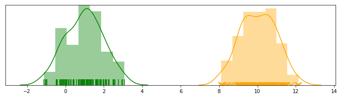
However, we may not know the real labels for each data point in reality. This, naturally, introduces a latent (a.k.a. hiddent/unobserved) variable called $\mathbf{z} = (z^{(1)}, …, z^{(m)})$, which is multinomial: $z^{(i)}$ indicates which distribution a specific point $x^{(i)}$ belongs to. In the example above, $z^{(i)}$ actually follows a Bernoulli, since there are only two possible outcomes.
In this case, we have a model: $p(\mathbf{x},\mathbf{z}; \Theta)$, where only $\mathbf{x}$ is observed. Our goal is to maximize $L(\Theta)=\prod_{i}p(x^{(i)};\Theta)$. It is common to instead maximize the log likelihood: $\ell(\Theta)=\sum_{i}ln~p(x^{(i)}; \Theta)$. This is also called the incompelte data log likelihood because we do not know the latent variable $\mathbf{z}$ that indicate each data point’s memebrship (to density which a data point belongs).
To gain more insights on why this problem is diffcult, we decompose the log likelihood:
Note that there is summation over $z^{(i)}$ inside logarithm. Even if individual joint probability distributions are in the exponential families, the summation still makes the derivative intractable.
Jensen Inequality
Before we talk about how EM algorithm can help us solve the intractability, we need to introduce Jensen inequality. This will be used later to construct a (tight) lower bound of the log likelihood.
Definition:
Let function $f$ be a convex function (e.g., $f’’ \geq 0$). Let $x$ be a random variable. Then we have $f(E[x]) \leq E[f(x)]$.
Further, $f$ is strictly convex if $f’’ > 0$. In such case, $f(E[x]) = E[f(x)]$ i.f.f. $x=E[x]$
On the other hand, $f$ is concave if $f’’ \leq 0$, and we have $f(E[x]) \geq E[f(x)]$.
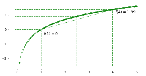
A useful example (that will be applied in EM algorithm) is $f(x) = ln~x$ is strictly concave for $x > 0$. Proof:
Therefore, we have $ln~E[x] \geq E[ln~x]$
Let’s go with a concrete example by plotting $f(x) = ln~x$
x = np.linspace(.1, 5, 100)
y = np.log(x)
fig, ax = plt.subplots(figsize=(8,4))
ax.scatter(x, y, color='green', marker='+')
## 1 (p=0.5)
ax.vlines(x=1, ymin=-2.5, ymax=0, linestyle='--', color='green')
ax.hlines(y=0, xmin=-.1, xmax=1, linestyle='--', color='green')
ax.text(x=1.1, y=np.log(.7), s='$f(1)=0$',
        fontdict={'size': 13})
## 4 (p=0.5)
ax.vlines(x=4, ymin=-2.5, ymax=np.log(4), linestyle='--', color='green')
ax.hlines(y=np.log(4), xmin=-.1, xmax=4, linestyle='--', color='green')
ax.text(x=4.1, y=np.log(3.1),
        s='$f(4)=%.2f$'%(np.log(4)),
        fontdict={'size': 13}
       )
ax.plot([1, 4], np.log([1, 4]), color='green', linestyle='dotted')
# E(x) = (1+4)/2 = 2.5
ax.vlines(x=2.5, ymin=-2.5, ymax=np.log(2.5), linestyle='--', color='green')
ax.hlines(y=np.log(2.5), xmin=-.1, xmax=2.5, linestyle='--', color='green')
EM Algorithm Formalization
Derivation
Now we can formarlize the problem, starting from the log likelihood from Section 1:
where $q_i(z^{(i)})$ is any arbitrary probability distribution for $z^{(i)}$ and thus:$q_i(z^{(i)}) \geq 0; \sum_{z^{(i)}}~q_i(z^{(i)}) = 1$.
It is interesting (actually important) to note that the summation inside the logarithm, $\sum_{z^{(i)}} q_i(z^{(i)}) \frac{p(x^{(i)}, z^{(i)}; \Theta)}{q_i(z^{(i)})}$, takes the form of expectation of $\frac{p(x^{(i)}, z^{(i)}; \Theta)}{q_i(z^{(i)})}$, given $x^{(i)}$. Recall that $E[f(x)] = \sum_i p(x^{(i)})f(x^{(i)})$, where $p(x)$ is the probability mass function for $x^{(i)}$. Therefore, we can write the above into:
Now, it is not difficult to see that we can apply Jensen Inequality on the term within the summation over $i$:
In this way, we successfully construct the lower bound for $\ell(\Theta)$. However, this is not enough. Note that we want to squeeze the lower bound as much as we can to obtain the equality. Based on Section 2, we need
where $c$ is some constant. And this leads to
From the formula above, we can determine the choice of $q$
The last term is actually the posterior distribution of $z^{(i)}$ (soft membership) given the observation $x^{(i)}$ and the paramter $\Theta$
Algorithm Operationalization
EM is an iterative algorithm that consists of two steps:
- E step: Let $q_i(z^{(i)}) = p(z^{(i)}\vert x^{(i)}; \Theta)$. The gives a tight lower bound for $\ell(\Theta)$. This is actually maximizing the expectation shown above.
- M step: Update parameters to maximize the lower bound $\Theta := argmax_{\Theta} \sum_i \sum_{z^{(i)}} q_i(z^{(i)})ln~\frac{p(x^{(i)}, z^{(i)}; \Theta)}{q_i(z^{(i)})}$
Convergence
To prove the convergence of EM algorithm, we can prove the fact that $\ell(\Theta^{(t+1)}) \geq \ell(\Theta^{(t)})$ for any $t$, where $\Theta^{(t)}$ is the parameter estimatations at iteration $t$.
Recall that we choose $q_i(z^{(i)}) = p(z^{(i)}\vert x^{(i)}; \Theta)$ so that Jensen inequality will become equality such that:
In the M step, we then update our parameter to be $\Theta^{(t+1)}$ that maximizes the R.H.S. of the equation above:
Therefore, EM algorithm will make the log likelihood change monotonically. A common practice to monitor the convergence is to test if the difference of log likelihoods at two success iterations is less than some predefined tolerance parameter.
Towards deeper understanding of EM: Evidence Lower Bound (ELBO)
We just derived the formulation of EM algorithm in details. However, one thing we did not do is to explicitly write out the decomposition of $\ell(\Theta)$. In fact, we can mathematically write out the log likelihood into the sum of two terms:
- $KL(q\vert \vert p) = \sum_{z} q(z) ln~ \frac{q(z)}{p(z \vert \mathbf{x}; \Theta)}$
- $\mathcal{L}(\mathbf{x}; \Theta) = \sum_{z} q(z) ln~ \frac{p(\mathbf{x}, z; \Theta)}{q(z)}$
Derivation
ELBO
Here, we define evidence lower bound to be $ELBO = \mathcal{L}(\mathbf{x}; \Theta)$, because KL-divergence is non-negative. Specifically, the equality only holds when $q(z) = p(z \vert \mathbf{x}; \Theta)$. Therefore, $ELBO$ can be seen as a tight lower bound of the evidence (incomplete data likelihood):
Such result is actually consistent with the previous derivation where we directly apply Jensen’s inequality.
Applying EM on Gaussian Mixtures
In this section, we will use an example of Gaussian Mixture to demonstrate the application of EM algorithm.
Suppose we have some data $\mathbf{x}={x^{(1)}, …, x^{(m)}}$, which some from $K$ different Gaussian distributions ($K$ mixtures). We will use the following notations:
- $\mu_k$: the mean of the $k^{th}$ Gaussian component
- $\Sigma_k$: the covariance matrix of the $k^{th}$ Gaussian component
- $\phi_k$: the multinomial parameter of a specific datapoint belonging to the $k^{th}$ componenet.
- $z^{(i)}$: the latent variable (multinomial) for each $x^{(i)}$
We also assume that the dimension of each $x^{(i)}$ is $n$.
The goal is: $max_{\mu, \Sigma, \phi}~ln~p(\mathbf{x};\mu, \Sigma, \phi)$. Therefore this follows exactly the EM framework.
E step
We set $w_j^{(i)} = q_i(z^{(i)}=j) = p(z^{(i)}=j \vert x^{(i)}; \mu, \Sigma, \phi)$.
M step
We will write down the lower bound and get derivatives for each of the three parameters.
Note that:
- $x^{(i)} \vert z^{(i)}=j; \mu, \Sigma \sim \mathcal{N}(\mu_j, \Sigma_j)$
- $z^{(i)}=j; \phi \sim Multi(\phi)$
We can then leverage these probability distributions and continue
Now, we need to maximize this lower bound for each of the three parameters. Many of the derivative on vector/matrix are based on Matrix Cookbook
Derivative of $\mu_j$
Set the last term zero, we have
Derivative of $\Sigma_j$
First, we consider the derivative of the first term in the square bracket:
Then, we do the second term
Combined these results back and set it to zero, we have:
Rearrange the equation and we have:
Derivative of $\phi_j$
This is relatively simpler but we need to apply Lagrange multipliers because $\sum_j \phi_j = 1$.
We need to construct Lagrangian, with $\lambda$ as the Lagrange multiplier:
We will take derivative on $\mathcal{L}$ and set it to zero:
Rearrange and we will have $\phi_j = -\frac{\sum_i w_j^{(i)}}{\lambda}$. Recall that $\sum_j \phi_j = 1$, we have:
Finally, we have:
Real example
class GMM(object):
    def __init__(self, X, k=2):
        # dimension
        X = np.asarray(X)
        self.m, self.n = X.shape
        self.data = X.copy()
        # number of mixtures
        self.k = k

    def _init(self):
        # init mixture means/sigmas
        self.mean_arr = np.asmatrix(np.random.random((self.k, self.n)))
        self.sigma_arr = np.array([np.asmatrix(np.identity(self.n)) for i in range(self.k)])
        self.phi = np.ones(self.k)/self.k
        self.w = np.asmatrix(np.empty((self.m, self.k), dtype=float))
        #print(self.mean_arr)
        #print(self.sigma_arr)

    def fit(self, tol=1e-4):
        self._init()
        num_iters = 0
        ll = 1
        previous_ll = 0
        while(ll-previous_ll > tol):
            previous_ll = self.loglikelihood()
            self._fit()
            num_iters += 1
            ll = self.loglikelihood()
            print('Iteration %d: log-likelihood is %.6f'%(num_iters, ll))
        print('Terminate at %d-th iteration:log-likelihood is %.6f'%(num_iters, ll))

    def loglikelihood(self):
        ll = 0
        for i in range(self.m):
            tmp = 0
            for j in range(self.k):
                #print(self.sigma_arr[j])
                tmp += sp.stats.multivariate_normal.pdf(self.data[i, :],
                                                        self.mean_arr[j, :].A1,
                                                        self.sigma_arr[j, :]) *\
                       self.phi[j]
            ll += np.log(tmp)
        return ll

    def _fit(self):
        self.e_step()
        self.m_step()

    def e_step(self):
        # calculate w_j^{(i)}
        for i in range(self.m):
            den = 0
            for j in range(self.k):
                num = sp.stats.multivariate_normal.pdf(self.data[i, :],
                                                       self.mean_arr[j].A1,
                                                       self.sigma_arr[j]) *\
                      self.phi[j]
                den += num
                self.w[i, j] = num
            self.w[i, :] /= den
            assert self.w[i, :].sum() - 1 < 1e-4

    def m_step(self):
        for j in range(self.k):
            const = self.w[:, j].sum()
            self.phi[j] = 1/self.m * const
            _mu_j = np.zeros(self.n)
            _sigma_j = np.zeros((self.n, self.n))
            for i in range(self.m):
                _mu_j += (self.data[i, :] * self.w[i, j])
                _sigma_j += self.w[i, j] * ((self.data[i, :] - self.mean_arr[j, :]).T * (self.data[i, :] - self.mean_arr[j, :]))
                #print((self.data[i, :] - self.mean_arr[j, :]).T * (self.data[i, :] - self.mean_arr[j, :]))
            self.mean_arr[j] = _mu_j / const
            self.sigma_arr[j] = _sigma_j / const
        #print(self.sigma_arr)
Setup dataset.
X = np.random.multivariate_normal([0, 3], [[0.5, 0], [0, 0.8]], 20)
X = np.vstack((X, np.random.multivariate_normal([20, 10], np.identity(2), 50)))
X.shape
(70, 2)
gmm = GMM(X)
gmm.fit()
Iteration 1: log-likelihood is -396.318688
Iteration 2: log-likelihood is -358.902036
Iteration 3: log-likelihood is -357.894632
Iteration 4: log-likelihood is -353.797418
Iteration 5: log-likelihood is -332.842685
Iteration 6: log-likelihood is -287.787552
Iteration 7: log-likelihood is -277.701280
Iteration 8: log-likelihood is -268.521010
Iteration 9: log-likelihood is -249.376342
Iteration 10: log-likelihood is -230.906536
Iteration 11: log-likelihood is -230.883025
Iteration 12: log-likelihood is -230.883025
Terminate at 12-th iteration:log-likelihood is -230.883025
gmm.mean_arr
matrix([[-0.05739539,  2.69216832],
        [20.04929409,  9.69219807]])
gmm.sigma_arr
array([[[0.30471149, 0.27830426],
        [0.27830426, 1.3309902 ]],

       [[0.94378014, 0.07495073],
        [0.07495073, 1.13089165]]])
gmm.phi
array([0.28571429, 0.71428571])

Zhiya Zuo
Filet-O-Fish 🍔 is the BEST!