Guassian Approximation to Binomial Random Variables

Saturday. March 03, 2018

I was reading a paper on collapsed variational inference to latent Dirichlet allocation, where the classic and smart Gaussian approximation to Binomial variables was used to reduce computational complexity. It has been a long time since I first learnt this technique in my very first statistics class and I would like to revisit this idea.

import numpy as np
import scipy as sp

import seaborn as sns
from matplotlib import pyplot as plt
%matplotlib inline

Single coin flip

I always feel like the example of coin flipping is used so much. Yet, it is simple and intuitive for understanding some (complex) concepts.

Let’s say we are flipping a coin with a probability of $p$ to get a head ($H$) and $1-p$ to get a tail (T). The outcome $X$ is thus a random variable that can only have two possible values: $X \in {H, T}$. For simplicity, we can use $0$($1$) to denote $T$($H$). In this case, we say that $X$ follows a Bernoulli distribution:

$$X \sim Bernoulli(p)$$

We can write the probability mass function as:

$$p(X=x) = p^x (1-p)^{1-x}, x\in \{0, 1\}$$

Then according to the defintions of expectation and variance, we have

\begin{align} E[X] &= \sum_{x \in \{0,1\}} p(X=x) = p^0 (1-p)^{1} + p^1 (1-p)^{1} = p \\ V[X] &= E[X^2] - E^2[X] = p - p^2 = p(1-p) \end{align}

Repetitive coin flips

How about we extend the above experiment a bit simply by doing that over and over gain? If we define a random variable $Y$ to denote the number of $1$’s across $n$ coin flips, we say $Y$ follows a Binomial distribution such that:

$$p(Y=k) = \binom{n}{k} p^k (1-p)^{n-k}$$

where $k$ is the number of $1$’s. The coefficient indicates the possible permutations of $0$’s and $1$’s in the final outcome. note that we can write $Y = \sum_i X_i$ since $X_i \in {0,1}$

It’s not difficult to get $E[Y]$ and $V[Y]$ by linearity of expectation and variance.

\begin{align} E[Y] &= E\Big[\sum_i X_i\Big] = \sum_i E[X_i] = \sum_i p = np \\ V[Y] &= V\Big[\sum_i X_i\Big] = \sum_i V[X_i] = \sum_i p(1-p) = np(1-p) \\ \end{align}

Visualization of $Y$

I like visualizations, because they help me better feel such abstract concepts. Let’s use an example of $(n, p)$ to see what Binomial distribution ($Y$) really looks like. Specifically, we will vary $n$ and see how the shape of the distribution may differ.

n_list = [10, 30, 50]
p = 0.3
k_list = [np.arange(0, n+1) for n in n_list] # support of Y

fig, ax = plt.subplots(figsize=(8,5))
for i, n in enumerate(n_list):
    pmf = sp.stats.binom.pmf(k_list[i], n, p)
    _ = ax.bar(k_list[i], pmf, alpha=.6, label='n=%d'%n)
_ = ax.legend()

png

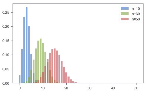
It seems like when $n$ goes larger, the distribution gets more symmetric. This, at least to me, is some kind of visual evidence that Gaussian approximation may actually work when $n$ is large enough.

Central limit theorem (CLT)

CLT is amazing! It implies that no matter what type of distributions we are working with, we can apply things that will work for Gaussian distributions to them. Specifically, I quote the first paragraph in Wiki below:

In probability theory, the central limit theorem (CLT) establishes that, in most situations, when independent random variables are added, their properly normalized sum tends toward a normal distribution (informally a “bell curve”) even if the original variables themselves are not normally distributed. The theorem is a key concept in probability theory because it implies that probabilistic and statistical methods that work for normal distributions can be applicable to many problems involving other types of distributions.

In the context of Binomial and Bernoulli random variables, we know that $Y = \sum_i X_i$. According to CLT, we have the following distribution:

$$\sqrt{n}~(\frac{Y}{n} - E[X]) \sim \mathcal{N}(0, V[X])$$

Combined with the equations above, we have:

\begin{align} \sqrt{n}~(\frac{Y}{n} - p) &\sim \mathcal{N}(0, p(1-p)) \\ \frac{Y-np}{\sqrt{n}} &\sim \mathcal{N}(0, p(1-p)) \\ Y &\sim \mathcal{N}(np, np(1-p)) \end{align}

Validation

Up to this point, we see that $Y \sim Binomial(n, p)$ can be approximated by $\mathcal{N}(np, np(1-p))$ given a relatively large number of $n$. Let’s try different $n$’s to see how well such approximation can perform!

n_list = [1, 3, 7, 10]
p = 0.7
k_list = [np.arange(1, n+1) for n in n_list]
x_list = [np.linspace(-2, 2*n, 1000) for n in n_list]

fig, ax_list = plt.subplots(nrows=1, ncols=len(n_list), 
                            figsize=(4*len(n_list), 3))
for i, n in enumerate(n_list):
    ax = ax_list[i]
    binom_p = sp.stats.binom.pmf(k_list[i], n, p)
    gauss_p = sp.stats.norm.pdf(x_list[i], n*p, n*p*(1-p))
    ax.bar(k_list[i], binom_p, color='seagreen',
           alpha=.6, label='Binomial')
    ax.plot(x_list[i], gauss_p, label='Gaussian', 
            color='seagreen')
    ax.set_title('$n=%d$'%n)
ax.legend()
fig.tight_layout()

png

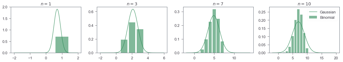
Now we can actually see that it is pretty good!

Zhiya Zuo

Filet-O-Fish 🍔 is the BEST!