Linear Regression Diagnostic in Python with StatsModels
import numpy as np
import statsmodels
import seaborn as sns
from matplotlib import pyplot as plt
%matplotlib inline
While linear regression is a pretty simple task, there are several assumptions for the model that we may want to validate. I follow the regression diagnostic here, trying to justify four principal assumptions, namely LINE in Python:
- Lineearity
- Independence (This is probably more serious for time series. I’ll pass it for now)
- Normality
- Equal variance (or homoscedasticity)
I learnt this abbreviation of linear regression assumptions when I was taking a course on correlation and regression taught by Walter Vispoel at UIowa. Really helped me to remember these four little things!
In fact, statsmodels itself contains useful modules for regression diagnostics. In addition to those, I want to go with somewhat manual yet very simple ways for more flexible visualizations.
Linear regression
Let’s go with the depression data. More toy datasets can be found here. For simplicity, I randomly picked 3 columns.
> df = statsmodels.datasets.get_rdataset("Ginzberg", "car").data
> df = df[['adjdep', 'adjfatal', 'adjsimp']]
> df.head(2)
| adjdep | adjfatal | adjsimp | |
|---|---|---|---|
| 0 | 0.41865 | 0.10673 | 0.75934 |
| 1 | 0.51688 | 0.99915 | 0.72717 |
Linear regression is simple, with statsmodels. We are able to use R style regression formula.
> import statsmodels.formula.api as smf
> reg = smf.ols('adjdep ~ adjfatal + adjsimp', data=df).fit()
> reg.summary()
| Dep. Variable: | adjdep | R-squared: | 0.433 |
|---|---|---|---|
| Model: | OLS | Adj. R-squared: | 0.419 |
| Method: | Least Squares | F-statistic: | 30.19 |
| Date: | Tue, 01 May 2018 | Prob (F-statistic): | 1.82e-10 |
| Time: | 21:56:07 | Log-Likelihood: | -35.735 |
| No. Observations: | 82 | AIC: | 77.47 |
| Df Residuals: | 79 | BIC: | 84.69 |
| Df Model: | 2 | ||
| Covariance Type: | nonrobust |
| coef | std err | t | P>|t| | [0.025 | 0.975] | |
|---|---|---|---|---|---|---|
| Intercept | 0.2492 | 0.105 | 2.365 | 0.021 | 0.039 | 0.459 |
| adjfatal | 0.3845 | 0.100 | 3.829 | 0.000 | 0.185 | 0.584 |
| adjsimp | 0.3663 | 0.100 | 3.649 | 0.000 | 0.166 | 0.566 |
| Omnibus: | 10.510 | Durbin-Watson: | 1.178 |
|---|---|---|---|
| Prob(Omnibus): | 0.005 | Jarque-Bera (JB): | 10.561 |
| Skew: | 0.836 | Prob(JB): | 0.00509 |
| Kurtosis: | 3.542 | Cond. No. | 5.34 |
Regression assumptions
Now let’s try to validate the four assumptions one by one
Linearity & Equal variance
Both can be tested by plotting residuals vs. predictions, where residuals are prediction errors.
> pred_val = reg.fittedvalues.copy()
> true_val = df['adjdep'].values.copy()
> residual = true_val - pred_val
> fig, ax = plt.subplots(figsize=(6,2.5))
> _ = ax.scatter(residual, pred_val)
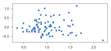
It seems like the corresponding residual plot is reasonably random. To confirm that, let’s go with a hypothesis test, Harvey-Collier multiplier test, for linearity
> import statsmodels.stats.api as sms
> sms.linear_harvey_collier(reg)
Ttest_1sampResult(statistic=4.990214882983107, pvalue=3.5816973971922974e-06)
Several tests exist for equal variance, with different alternative hypotheses. Let’s go with Breusch-Pagan test as an example. More can be found here. Small p-value (pval below) shows that there is violation of homoscedasticity.
> _, pval, __, f_pval = statsmodels.stats.diagnostic.het_breuschpagan(residual, df[['adjfatal', 'adjsimp']])
> pval, f_pval
(6.448482473013975e-08, 2.21307383960346e-08)
Usually assumption violations are not independent of each other. Having one violations may lead to another. In this case, we see that both linearity and homoscedasticity are not met. Possible data transformation such as log, Box-Cox power transformation, and other fixes may be needed to get a better regression outcome.
Normality
We can apply normal probability plot to assess how the data (error) depart from normality visually:
> import scipy as sp
> fig, ax = plt.subplots(figsize=(6,2.5))
> _, (__, ___, r) = sp.stats.probplot(residual, plot=ax, fit=True)
> r**2
0.9523990893322951
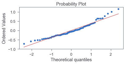
The good fit indicates that normality is a reasonable approximation.

Zhiya Zuo
Filet-O-Fish 🍔 is the BEST!