Plot Lorenz Curve in Python
import numpy as np
from matplotlib import pyplot as plt
%matplotlib inline
Gini coefficient, along with Lorenz curve, is a great way to show inequality in a series of values. However, there are no straight forward wrapper function to use for the plot. I’ve been using these a lot lately and woud like to write down how I do these with Numpy and Matplotlib.
Let’s first come up with a small sample set. To make a skewed dataset, I append two Poisson random samples together.
X = np.append(np.random.poisson(lam=10, size=40),
              np.random.poisson(lam=100, size=10))
X
array([ 11,  11,  13,  10,  17,  14,  14,   9,   8,  11,   4,  13,  12,
         9,  14,  11,  10,  11,  13,  17,  14,   6,  10,   8,  13,  14,
        13,   5,  22,   8,  13,  10,  11,  14,   6,   6,  11,  10,   6,
         7, 103,  86,  99,  94,  99,  95,  91,  95,  88,  79])
Calculation of Gini
The formula comes from Gini’s Wikipedia page:
Note that the values of $y$’s are ordered such that $y_i \leq y_{i+1}$
Now, we can write a simple wrapper function for this.
def gini(arr):
    ## first sort
    sorted_arr = arr.copy()
    sorted_arr.sort()
    n = arr.size
    coef_ = 2. / n
    const_ = (n + 1.) / n
    weighted_sum = sum([(i+1)*yi for i, yi in enumerate(sorted_arr)])
    return coef_*weighted_sum/(sorted_arr.sum()) - const_
gini(X)
0.5305263157894735
Lorenz Curve
There are two elements we need: perfect equality that has a slope of $1$ and the Lorenz curve.
Quote from Lorenz curve’s wiki page
The curve is a graph showing the proportion of overall income or wealth assumed by the bottom $x$% of the people
In fact, the famous 80-20 rule is one good example: the bottom 80% holds 20% of the overall wealth. Under the situation of perfect equality, on the other hand, we can say the bottom $x$% holds $x$% of the overall wealth.
Similar to Gini coefficient, we will sort the data. Then we convert values to cumulative proportions. We may also add the origin $(0,0)$
X_lorenz = X.cumsum() / X.sum()
X_lorenz = np.insert(X_lorenz, 0, 0)
X_lorenz[0], X_lorenz[-1]
(0.0, 1.0)
fig, ax = plt.subplots(figsize=[6,6])
## scatter plot of Lorenz curve
ax.scatter(np.arange(X_lorenz.size)/(X_lorenz.size-1), X_lorenz,
           marker='x', color='darkgreen', s=100)
## line plot of equality
ax.plot([0,1], [0,1], color='k')
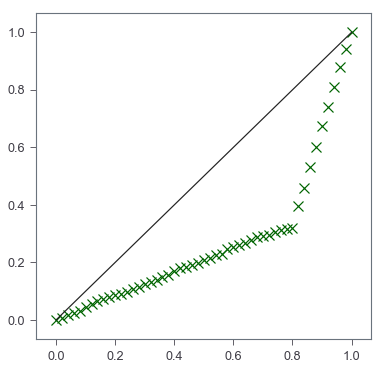
This gives us a very simple Lorenz curve. Then it is up to our own needs to add any customization.
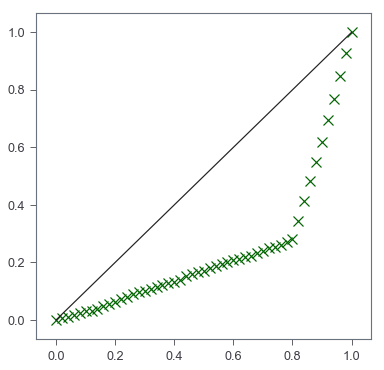
A wrapper function
def lorenz_curve(X):
    X_lorenz = X.cumsum() / X.sum()
    X_lorenz = np.insert(X_lorenz, 0, 0)
    X_lorenz[0], X_lorenz[-1]
    fig, ax = plt.subplots(figsize=[6,6])
    ## scatter plot of Lorenz curve
    ax.scatter(np.arange(X_lorenz.size)/(X_lorenz.size-1), X_lorenz,
               marker='x', color='darkgreen', s=100)
    ## line plot of equality
    ax.plot([0,1], [0,1], color='k')
X = np.append(np.random.poisson(lam=10, size=40),
              np.random.poisson(lam=100, size=10))
gini(X)
0.5620936639118459
lorenz_curve(X)

Zhiya Zuo
Filet-O-Fish 🍔 is the BEST!